 Map displaying the Storm Prediction Center (SPC) Convective Outlook issued at 8:00 am CDT March 25, 2015, and preliminary reports of tornadoes (red dots), large hail (green dots), and strong winds (blue dots) for the period of 8:00 am March 25 to 7:00 am CDT March 26, 2015. Note that the reports have not been filtered for duplicates. Image source NOAA/Storm Prediction Center
On March 25, 2015, a round of severe thunderstorms struck portions of the Southern Plains and Ozark Mountains after a surprisingly tornado-free first 24 days of the month.
The storms spawned at least eight tornado reports as of this writing – three in northwestern Arkansas, three in northeastern Oklahoma near Tulsa, and at least two in the Oklahoma City suburb of Moore – along with at least 178 reports of large hail and 52 reports of strong, damaging winds.
A map displaying the preliminary reports overlaid on the Storm Prediction Center (SPC) Convective Outlook issued that afternoon is found above and a radar loop of a portion of the event, with warnings superposed, is found below.
In this post, I’ll examine the meteorology behind these storms and tornadoes, particularly the tornadoes that hit portions of Moore.
 Southern Plains radar composite for the time period 5:30 – 8:25 pm CDT March 25. Tornado (red), severe thunderstorm (blue) and flash flood (green) warnings are superposed on the radar image. Image source WeatherBell
On the afternoon of March 25, a stalled front over Oklahoma and Arkansas was forecast to move southward as a cold front and provide the focus for thunderstorm formation.
Surface weather map valid 4 p.m. CDT on March 25. courtesy NOAA/Weather Prediction Center.
Ample instability – measured by the convective available potential energy (CAPE) – existed along and south of this front (below), with values ranging from 2000 to over 3000 J/kg.
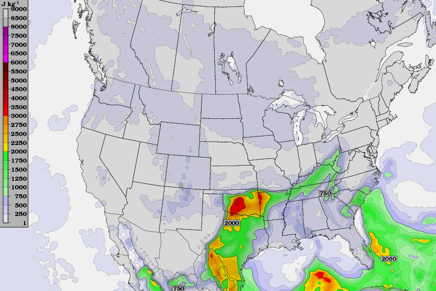
CAPE (J/kg) at 4 p.m. CDT March 25. Image courtesy TwisterData.
Deep-layer vertical wind shear – defined as the change in wind speed or direction within the lowest 6 km or 3.5 miles of the atmosphere – was also more than sufficient for storm organization and rotation.
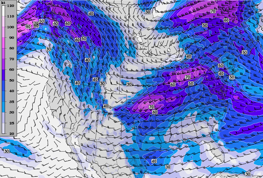
Deep-layer vertical wind difference (knots) at 4 p.m. CDT March 25. Image courtesy TwisterData.
This meant that all of the ingredients for severe weather – instability, vertical wind shear, and a trigger – were in place for severe weather, and the SPC in Norman, OK, issued a moderate risk for severe thunderstorms.
Aside from the ingredients mentioned above, research has also determined that strong, long-lived tornadoes also require strong wind shear in the first kilometer (3,000 feet) above ground level, as well as high surface relative humidity. Neither of these were forecast to be particularly favorable for tornadoes on this day. A further concern was storm mode, or type, since discrete supercell thunderstorms are far more likely to produce tornadoes than lines or clusters of storms. Mixed-mode cases such as this, particularly those forming along cold fronts, continue to present one of the greatest challenges to tornado forecasters.
High-resolution numerical model output – capable of resolving individual thunderstorms – can offer insights into the storm mode, but cannot, and should not, be taken as gospel. One such forecast is reproduced below and depicts a mixed mode of storms – a line of storms with embedded circulations. Further analysis of the conditions revealed that as the storms formed along the front, they would likely become undercut by the front as the front pushed southward (imagine storms moving parallel to the front above, but as the front pushes southward, the storms end up on the cool (north) side of the front).
Such storms are known to forecasters as “elevated thunderstorms” and are unlikely to produce tornadoes.
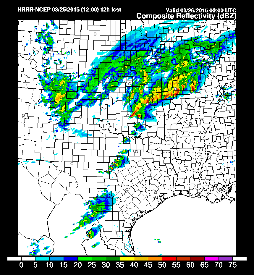
Simulated radar reflectivity from the high-resolution rapid refresh (HRRR) model for 7:00 pm CDT March 25 (0000 UTC March 26). Image courtesy NOAA/Earth Systems Research Laboratory.
Given all of these environmental factors, the SPC maintained a 5% chance of tornadoes within 25 miles of a point in the moderate risk area (a fairly low tornado probability for a moderate risk), and stressed large hail as the dominant thunderstorm hazard.
Accordingly, a severe thunderstorm watch was issued at 2:15 pm CDT for Central and Eastern Oklahoma, Northwestern Arkansas, and adjacent portions of Kansas and Missouri. The watch text states that there was a 20% chance of two or more tornadoes occurring in this area, which is a fairly high probability for a severe thunderstorm watch. My personal analysis of the set up agreed with this forecast – there might be a weak tornado or two – I’d consider chasing if it was in my backyard, but it was not something that I’d drive 10 hours from Illinois to Oklahoma to witness.
So given this detailed analysis, why were there so many tornadoes?
The tornadoes that occurred on March 25 were generally weak and short lived. Please keep in mind that a weak tornado may still contain winds over 100 mph – easily capable of blowing down trees, lofting debris, flipping mobile homes, and rolling over vehicle – and is still dangerous.
The most photographed, and likely most intense (given a preliminary rating of EF-2 by the National Weather Service in Tulsa) tornado of the day, occurred near Sand Springs, OK, just west of Tulsa. This tornado was responsible for considerable damage and unfortunately one fatality in the Riverside Mobile Home Park in Sand Springs. It is worth stating again that tornadoes are in no way attracted to mobile home parks, but the inferior construction endemic to mobile homes means that tornado damage and tornado casualties disproportionately occur in mobile home communities. The picture below reiterates just how vulnerable mobile homes are to tornadoes.
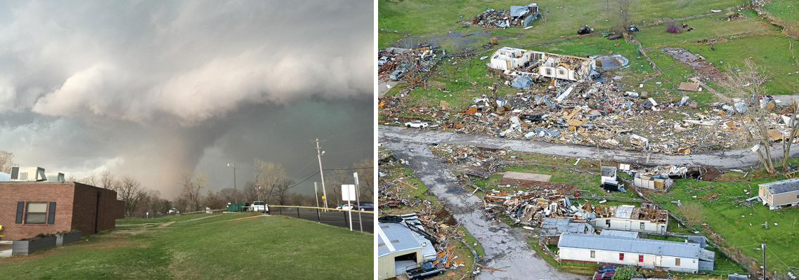
Photo of the Sand Springs, OK, tornado (left) via Chris Young and damage to the Riverside Mobile Home Park (right) via Tulsa World.
This tornado also caused extensive damage to, among other structures, a donut shop and a gymnastics studio. Fortunately, the gymnastics studio owner reviewed her weather safety plan that morning and got all of her students to shelter when the warning was issued. There were no injuries at that location. Her actions stand as a shining example of how to be prepared for severe weather.
The region of Northeastern Oklahoma and Northwestern Arkansas – where most of the tornadoes occurred – was most vulnerable to tornadoes owing to a surface boundary over the region (see surface analysis below).
Related: Forecasting tornadoes? Look for boundaries
The storms that affected this region formed earlier in the afternoon along and ahead of the surface cold front near Oklahoma City. These storms did not produce any tornadoes until they interacted with this secondary boundary over Northeastern Oklahoma and Northwestern Arkansas. This boundary was a stalled cold front that had produced severe storms in Missouri the previous day and had been reinforced by thunderstorm outflow (cold air that rushes out of thunderstorms) earlier that afternoon.
With the exception of the Moore tornadoes, all of the other tornadoes occurred along or near the purple line in the image below. The right image below also reveals enhanced low-level shear in the immediate vicinity of this boundary, a crucial ingredient for tornadoes.
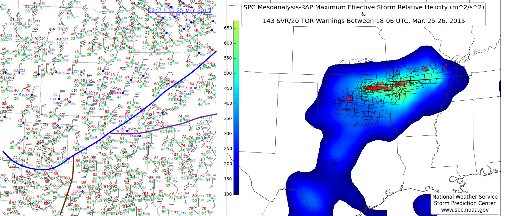
Left: Surface analysis from 5:43 pm CDT. The blue line indicates the surface cold front, the brown line indicates the surface dryline, and the purple line indicates the secondary boundary that was likely instrumental to the tornadoes in Northeastern Oklahoma and Northwestern Arkansas. Image courtesy UCAR/RAP, analysis by the author. Right: Analysis of maximum effective storm-relative helicity (low-level vertical wind shear) between 1:00 pm March 25 and 1:00 am CDT March 26. Tornado warnings are red-shaded polygons and severe thunderstorm warnings are black outlines. Image courtesy Greg Carbin/NOAA/SPC
The cause of the tornadoes near Moore is a bit different. Notice that there is no secondary boundary in Central Oklahoma with which the storms can interact.
In this case, it was a smaller-scale (storm-scale) interaction that led to these tornadoes. A series of radar images shown below illustrates how the parent supercell thunderstorm, which had been undercut by the cold front as forecast, sucked the cold front back toward it (at this point, the cold front had also been reinforced by thunderstorm outflow, and is referred to as a composite boundary).
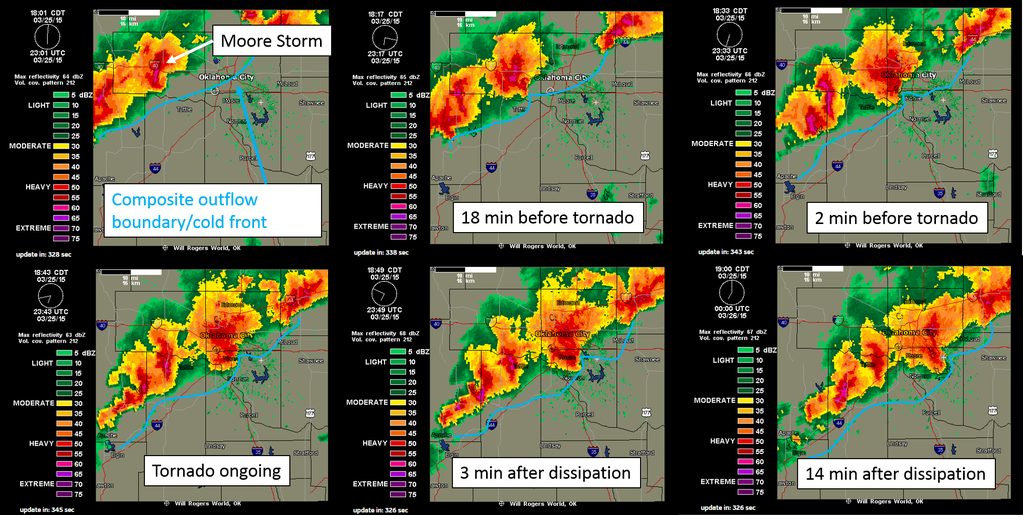
Series of radar reflectivity images around the time of the Moore tornado. The boundary is annotated in light blue. Radar images courtesy Weather Underground, analysis and annotation by the author.
This series of images reveals that, about a half hour prior to tornado formation, the supercell that would produce the tornadoes near Moore was located west of Oklahoma City, near El Reno. This storm was behind the cold front at this time, and it seemed unlikely that it would produce a tornado.
The storms to the immediate northeast and southwest of this one were much closer to the boundary and seemed to be better (albeit still not likely) candidates to produce tornadoes. By 6:17 p.m. CDT (top center), a kink formed in the boundary to the immediate southeast of the Moore storm as strong winds from the southeast flowing into the storm pulled the boundary back toward the storm. This kink became even more prominent by 6:33 p.m., two minutes prior to tornadogenesis, and remained in close proximity to the storm even after the tornado dissipated at 6:46 pm.
A closer examination of the Doppler velocity data provides more detail about the characteristics of the circulation and the reason for its eventual demise.
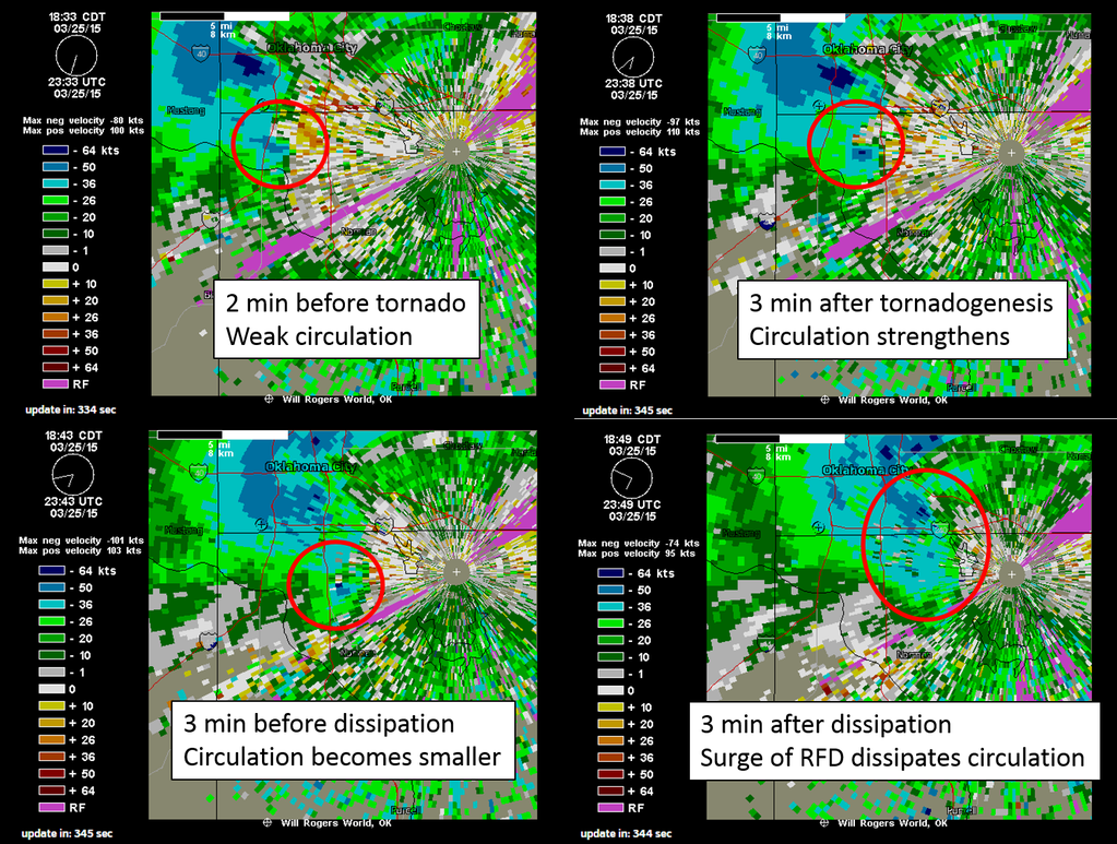
Series of Doppler velocity images around the time of the Moore tornado. Blue and green colors represent winds blowing toward the radar site (from the west in the area of the circulation); orange colors represent winds blowing away from the radar site (from the east in the area of the circulation). The circulation is circled in red. Images courtesy Weather Underground, annotation by the author.
A circulation is evident over southwestern portions of Oklahoma City two minutes prior to tornadogenesis. Circulations like this are not uncommon, however, along the leading edge of hook echoes of supercell thunderstorms. This circulation strengthened by 6:38 p.m. – three minutes after the first tornado had likely formed. The circulation became smaller as the tornado – or possibly a second tornado – persisted at 6:43 pm (again, the damage survey is still ongoing as of this writing). The final tornado dissipated at 6:46 pm as a rear-flank downdraft surge (the circled blue colors in the lower-right panel) disrupted and choked off this circulation. Strong RFD surges such as this were noted in many of the storms that afternoon, including those in the Tulsa area.
The strong RFD winds are also evident in these images. The light blue shading on the image represents winds greater than 36 knots (41 mph), the darker blue represents severe winds greater than 50 knots (58 mph), and the darkest blue indicates winds greater than 64 knots (75 mph).
Although no tornado warning was in place at the time this tornado formed, it is sometimes next to impossible to warn for every small-scale circulation. A severe thunderstorm warning was in effect, noting that golfball-sized hail and 70 mph winds were possible. This underscores the fact that people need to take severe thunderstorm warnings seriously as well, not just tornado warnings; I certainly would not want to be caught outside or in my car in conditions like that. There are also high-resolution radar loops of this storm, available from the Cooperative Institute for Mesoscale Meteorology Studies at the University of Oklahoma.
It is not uncommon for storm-boundary interactions such as this to produce tornadoes, although they are usually relatively weak tornadoes (but sill dangerous), as noted by the National Weather Service Forecast Office in Norman, OK. It is also important to note that not every such storm-boundary interaction produces a tornado. The storms to the immediate northeast and southwest of the Moore storm both failed to produce tornadoes. Also, Blanchard (2008) published a case of a storm pulling a boundary back toward it; this storm also failed to produce a tornado (h/t James Correia, Jr).
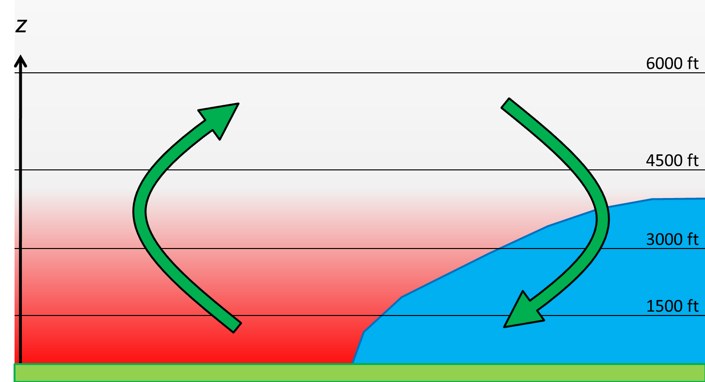
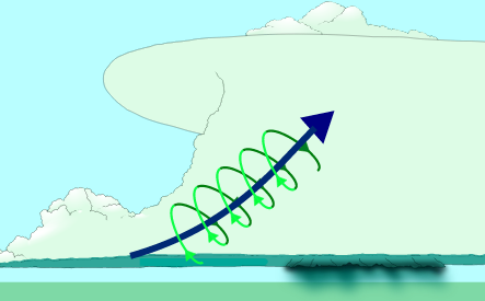 (Top): Schematic illustrating how a horizontal gradient in temperature can result in a horizontal circulation. Areas of warm air are shaded red and areas of cold air are shaded blue; temperature decreases with height in the warm air mass. The green arrows depict the resultant circulation. Image by the author. (Bottom): Illustration of tilting of horizontal rotation into the vertical by a storm’s updraft. Image credit Wikipedia
Boundaries such as these are regions of enhanced horizontal rotation, as seen in the diagram above. The air on the colder side of the boundary wants to sink and spread laterally along the surface, while the air on the warmer side of the boundary wants to rise up and over the colder air.
When thunderstorms encounter such regions of enhanced horizontal rotation, their updrafts can tilt this rotation into the vertical as seen in the bottom image, resulting in stronger vertical rotation at about 1000 feet above ground level. This stronger low-level circulation is far more efficient at sucking air upward, and can thus stretch and amplify rotation at the surface much faster, resulting in increased tornado potential. (A detailed post or posts on the current scientific understanding of the tornadogenesis process will be coming this summer.)
http://www.youtube.com/watch?v=B_4QE4EjrNA&feature=youtu.be
Video of the Moore, OK, tornado from KWTV-TV.
It is clear from this video and from the preliminary damage pictures below that this event was far different from the F5 tornado of May 3, 1999, or the EF5 tornado of May 20, 2013.
These latter cases were long-tracked, intense tornadoes that caused devastating damage across large swaths of the city, while the March 25 tornado was likely composed of multiple, short-lived, much weaker tornadoes, superposed with strong straight-line winds from the rear-flank downdraft, according to the NWS (the damage survey is still ongoing as of this writing, but has found at least EF-1 damage). Of course, all of this is small consolation to those who may have had their property damaged or suffered injuries in these storms.
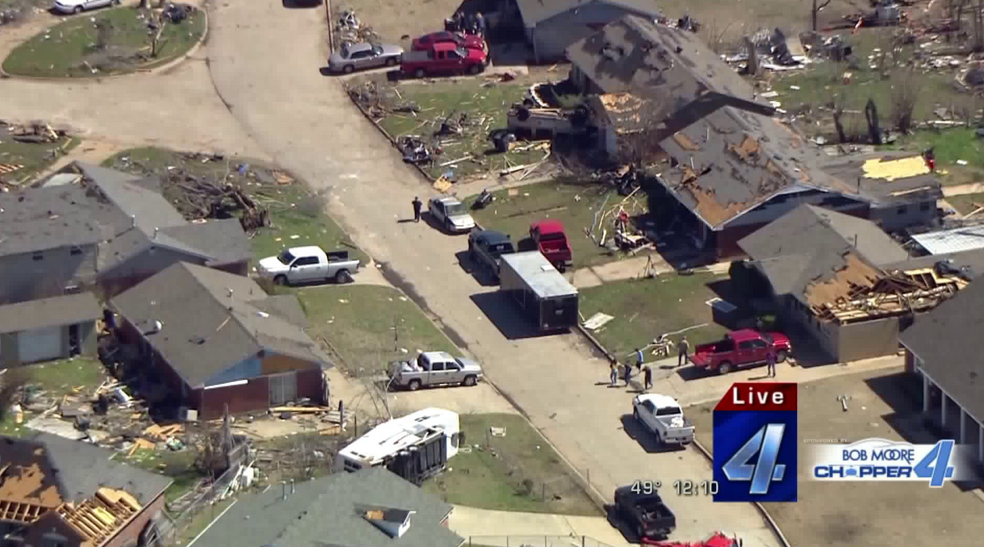
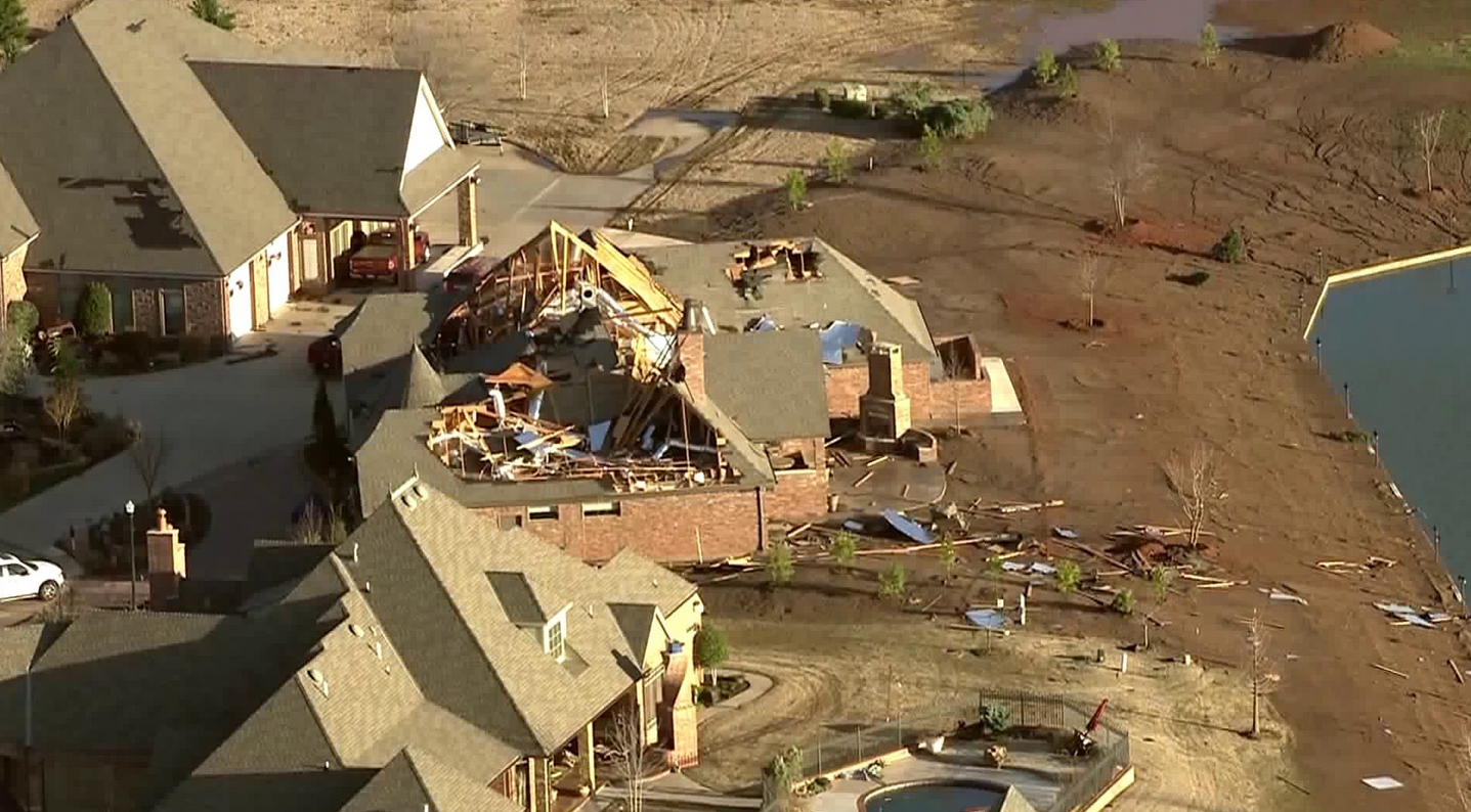
Aerial photos of tornado damage from the Moore, OK, tornado of March 25, 2015. Images courtesy KFOR-TV.
As the map below left illustrates, this is the fifth tornado to impact Moore since an F2 struck on October 4, 1998. The others were the devastating F5 that struck on May 3, 1999, the F4 of May 8, 2003, and the EF5 of May 20, 2013.
There is nothing scientifically significant about Moore that attracts tornadoes. It is not cursed, it is not because it is a suburb, or has open fields east of it or west of it. It is not because of its proximity to Oklahoma City. Indeed, the right image below indicates that the entire Oklahoma City metro area is no stranger to tornadoes, and this is simply owing to its geographical placement in the heart of tornado alley.
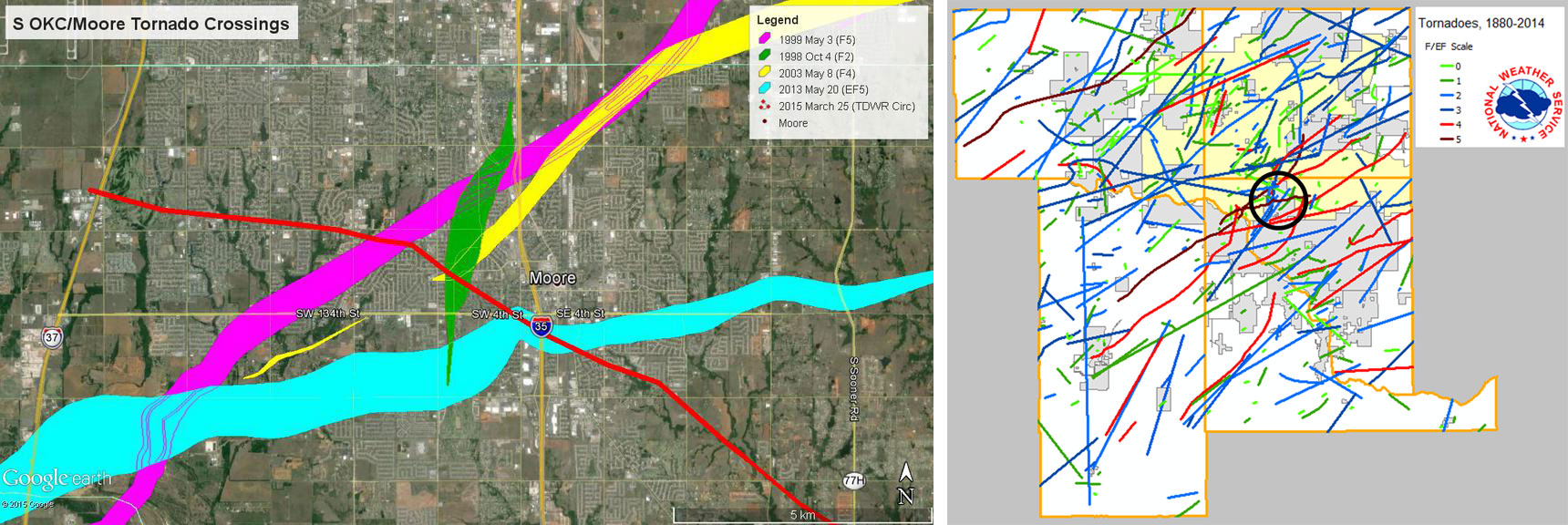 Left: Map of tornado tracks impacting Moore, OK, and surrounding areas from 1998-2015. Image courtesy Kiel Ortega/CIMMS/OU. Right: Map of tornadoes impacting the Oklahoma City metropolitan area from 1880-2014. Moore is circled in black. Map courtesy Rick Smith/NOAA/NWS Norman.
In summary, severe thunderstorms spawned several relatively brief tornadoes across portions of Oklahoma and Arkansas on May 25, 2015. Based on the analyses presented above, it is likely that storm-boundary interactions were crucial in the formation of most, if not all, of these tornadoes. The storms exhibited mixed mode characteristics as expected; additionally, the storms had trouble containing their outflow owing to the relatively small values of low-level shear and the mixed-mode characteristics exhibited. Had this not been the case, the tornado threat, and likely the damage, could have been far worse.
Great recap! A friend of mine was on the storm as it passed through Madison County in Northwest Arkansas. He did a post with some pics here: http://www.noiseblankers.com/frontpage/storm-hunting-with-k5kac.html
Nice pics – thanks for sharing!
Excellent analysis! A satellite perspective of these storms has been posted on the CIMSS Satellite Blog: http://cimss.ssec.wisc.edu/goes/blog/archives/17983
Very interesting – will share!
Thanks Jeff, this is a great recap and will be a great read for my Severe Wx forecasting students.
Chris – Great to hear; I may do the same.
i noticed both the Moore and the Sand Springs tornado path was to the SE. While I know that all tornadoes don’t follow a NE path it seems that few have a SE path. With both of these on the same day having a SE path I was wondering if something about the conditions caused that? Thanks for the informative article.
Glad you enjoyed it. Tornado motion is generally dictated by the motion of the parent supercell thunderstorm. Supercells usually move with, but just to the right of, the mean winds in the atmosphere (right is relative to an observer moving with the winds). In a lot of strong tornado environments, the mean winds are from the SW, resulting in a NE storm motion. On Wednesday, however, the upper-level flow was more from the due west, making storm motion more toward the east or even SE.
Also, you cannot judge the intensity of a tornado by its motion. For example, the May 20, 2013, Moore tornado moved toward the NE, but the May 31, 2013, El Reno tornado moved (erratically) toward the east.
Great write up and diagnosis.
One minor tweak, the gymnasium damage was caused by straight-line winds, estimated by the WCM at NWS Tulsa at 100mph. That manager is this storm’s hero. She had a plan, stayed weather aware, and executed the plan.
So why did NWS not issue a warning in Moore after numerous reports by trained spotters, notified them that there was a tornado on the ground, (first indication) or around the time the inflow notch developed and it was fairly evident there was low level circulation? (Second indication). I’m just confused because I thought warnings were issued when these events are imminent or occurring. Contrary to some people’s beliefs I feel all tornadoes should be warned.
James, thank you for the note on the gymnasium damage; I was unaware.
Bails, not every low-level circulation such as what was over Moore produces a tornado. I am not a warning forecaster, but I know it is an often difficult job; one wants to warn for every tornado before it touches down. On the flip side, one cannot warn for every potentially tornadic circulation or else the false alarm rate (warnings when there are no tornadoes) would be unacceptably high. Compounding this problem are the occasional false tornado reports (blowing dust, rain shafts, gustnadoes, etc., being reported as tornadoes) received by the NWS. It is obviously regrettable that no tornado warning was in place and I have already heard that the folks at NWS Norman will be investigating what transpired in those critical 10 minutes. I wish I could give you more information as to what happened, but I was not there.
Great article. Could you elaborate on the “secondary boundary” mentioned in the article for people like me who aren’t as meteorologically proficient as you? Thanks.
Don’t forget about the EF-4 that hit the SE part of Moore on May 10 2010
Trey, That secondary boundary was a cold front that fired storms over Missouri on Tues 3/24 http://www.spc.noaa.gov/climo/reports/150324_rpts.html. This front moved SE then stalled over OK/AR on Wednesday. Storms formed N of this boundary over KS/MO on Wed, and this reinforced the cold air N of it. You can follow the progression of this front here (click next map to jump ahead 3 h): http://www.hpc.ncep.noaa.gov/archives/web_pages/sfc/sfc_archive_maps.php?arcdate=03/24/2015&selmap=2015032421&maptype=namussfc. Hope this helps.
GDiamond – Good catch; the EF-4 hit far SE Moore; there was an EF-1 there too http://www.srh.noaa.gov/images/oun/wxevents/20100510/maps/Central.png
Thanks for your answer and the links. They were very insightful as was your whole article.
In addition to the five tornadoes that hit Moore mentioned above, May 10, 2010 saw an EF-4 go through South Moore with two EF-1 satellites.
A little late in replying, but I love this article as well as others of yours. A plethora of knowledge for those of us not in the field. Very informative and helpful!!!